Fault diagnosis in electric motors using multi-mode time series and ensemble transformers network
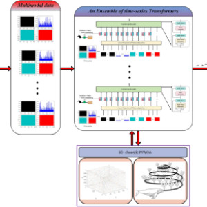
This section details the motor fault diagnosis method for the multi-modal time series based on ensemble Transformer networks. The overall structure, as shown in Fig. 4, mainly comprises a multi-modal data acquisition module, an ensemble Transformer network, classifier, etc. It is particularly crucial to note that the ensemble Transformer network is a parallel ensemble of multiple time-series Transformer networks.
Moreover, the performance of each time series Transformer network is influenced by its hype-parameters. Therefore, in order to enhance the network performance, a modified WOA algorithm is proposed in this section to identify the optimal hyper-parameters.
Fig.
4

Frame diagram of the proposed motor fault diagnosis algorithm.
Ensemble transformer network
Multi-modal time series possess diverse data structures and expressions, and a single Transformers network cannot comprehensively extract their features. Therefore, in this section, an innovative ensemble Transformer network is proposed, which assigns specialized Transformer networks to different modalities within the multi-modal time series, creating a parallel ensemble of multiple Transformer networks.
Figure 5 illustrates the overall architecture of the ensemble Transformer network. In Fig. 5a, the entire network is composed of multiple time series Transformer networks, Add & Norm modules and classifiers. Figure 5b provides a detailed view of the network structure for a single time series Transformer, which is designed to fully consider the characteristics of time series data and can effectively extract useful information from complex datasets.
Fig.
5

Transformers network structure. (a) Consolidated Transformers network. (b) Transformers network with a single time series.
The Multi-modal data acquisition module integrates multiple sensors and data acquisition techniques for simultaneous collection of different types of data, including sound, vibration, current, and other diverse data modes. The time-series Transformer networkdecomposes multidimensional time series into small, fixed-size patches, then linearly embeds them, adds positional embeddings, and feeds the resulting sequence of vectors into a standard Transformer encoder. For classification purposes, the standard approach is utilized here, which involves adding an additional learnable component, termed a ‘classification token,’ to the sequence.
The detailed structure is as follows: (1) Token embedding. The standard Transformer network receives one-dimensional sequences that are embedded as tokens.
However, the time series from different modalities within a multi-modal time series can be multidimensional, which is the case for time series data (x in {mathbb{R}}^{M times N times C}). Here, the M and N denote the length and dimension of the time series, respectively, and C represents the number of channels. Subsequently, the data is flattened to (x in {mathbb{R}}^{M times (N times C)}).
Moreover, it is divided along the time axis into A-block sequences (left[ {x^{1} ,x^{2} , cdots ,x^{M} } right]) and (x^{M} in {mathbb{R}}^{N times C}). A constant latent vector of size D is used in all layers of the Transformer. Consequently, the block sequence is augmented and mapped to dimension D by a trainable linear projection.
The output of this projection is referred to as the Token embedding. (2) Class token. Similar to BERT’s [class] token, adding a learnable embed ((z_{0}^{0} = x_{class})) to the block sequence (left[ {x^{1} ,x^{2} , cdots ,x^{M} } right]) results in a new embedded block sequence (z_{0} = left[ {x_{class} ;x^{1} E;x^{2} E; cdots ;x^{N} E} right]), where (E in {mathbb{R}}^{(N times C) times D}) C.
(3) Position embeddings. To preserve location information, position embeddings are added to the block sequence. Here, the standard learnable 1-D position embedding method is employed, and z0 is extended to obtain (z_{0} = left[ {x_{class} ;x^{1} E;x^{2} E; cdots ;x^{N} E} right] + E{}_{positon}), where (E_{postion} in {mathbb{R}}^{(N + 1) times D}).
The resulting sequence of embedding vectors is then used as input to the encoder. (4) Encoder. This section still utilizes the Transformer encoder, which is consists of N Transformer blocks and takes as input the embedding sequence z0.
Each Transformer block includes a Multi-Headed Self-Attention layer, an Add & Norm layer, and a Feed-Forward Neural Network layer. This can be expressed by the following formula: ££{text{z}}_{l}^{prime } = {text{LayerNorm}} (MSA(z_{l – 1} ) + z_{l – 1} )begin{array}{*{20}c} {} & {l = 1,2, cdots ,N} \ end{array}££
(10) ££{text{z}}_{l} = {text{LayerNorm}} (FFN(z^{prime}_{l} ) + z^{prime}_{l} )begin{array}{*{20}c} {} & {l = 1,2, cdots ,N} \ end{array}££ (11)
where, MSA(o) is a Multi-Headed Self-Attention layer; FFN(o) is a Feed-Forward Network layer. Moreover, due to the multi-modal time series, each time series data has its own range of features. Each encoder outputs a hidden state ({text{z}}_{l}^{c}) with a distinct range of values, and this diversity makes subsequent modules unstable.
Therefore, a context normalization model is introduced, which is defined as follows. ££{tilde{text{z}}}_{l}^{c} = frac{{z_{l}^{c} – mean(beta_{n} z_{l}^{c} )}}{{std(beta_{n} z_{l}^{c} )}}££ (12)
where, ? is a hyper-parameter that determines the weight of ({text{z}}_{l}^{c}). The Self-Attention layer can dynamically focus on specific modalities or points in time based on the importance of each mode at different times, which enables it to more effectively capture relevant information across modalities. However, self-attention has time and space complexity that is proportional to the sequence length, making it inefficient for lengthy sequences.
To enhance the efficiency of ensemble Transformer network, Learning-To-Hash Attention (LHA) is employed here as a replacement for self-attention. The core idea is to separate parameterized hash functions for query and key learning, allowing sparse pattern in LHA to adapt beyond distance-based hash functions such as (Locality Sensitive Hashing) LSH or online k-means, and to better align the mismatch between query and key distribution. The Sparse attention is defined as follows.
££tilde{H} = {text{Sparse}} – Attention(Q_{i} ,K,V) = sumlimits_{{j:h_{Q} (Q_{i} ) = h_{K} (Kj)}} {overline{A}_{ij} V_{j} }££ (13) where, (h_{K} ,h_{Q} :{mathbb{R}}^{{d_{h} }} mapsto left[ B right]) is the hash function of the key and query and B is the hash bucket. (overline{A}_{ij} propto A_{ij}) is the attention weight satisfying (forall i) and (sumnolimits_{{j:h_{Q} (Q_{i} ) = h_{K} (K_{j} )}} {overline{A}_{ij} } = 1).
By defining a parametrized function (H_{K} ,H_{Q} :{mathbb{R}}^{{d_{h} }} mapsto {mathbb{R}}^{B}), LHA implements a learnable hash function (h_{K} ,h_{Q} :{mathbb{R}}^{{d_{h} }} mapsto left[ B right]), as follows. ££h_{Q} (Q_{i} ) = mathop {argmax}limits_{{b in left{ {1,2, cdots ,B} right}}} left[ {H_{Q} (Q_{i} )} right]_{b}££ (14)
££h_{K} = mathop {argmax}limits_{{b in left{ {1,2, cdots ,B} right}}} left[ {H_{K} (K_{j} )} right]_{b}££ (15) where,(H_{Q}) and (H_{K}) are arbitrary parameterized functions.
Finally, a single linear layer is applied to obtain the hidden state (tilde{H}). The Add & Norm layer adds the hidden state output from the attention layer to the input, thereby preserving the original input information within the network and preventing information loss. The subsequent normalization step normalizes the results of this addition, aiding the network in converging more smoothly during training and enhancing the model’s generalization performance.
The Classifier constitutes the bottom layer of the ensemble Transformer network. Firstly, each time series Transformer is employed to encode and generate a feature representation of the input data. These features encapsulate contextual information about the input data.
Secondly, the classifier tmaps the features from the output of the additive-forward multi-layer perceptron (MLP) through the activation function, specifically Softmax, to the probability distribution of the class categories, as follows: ££Class(z_{N}^{0} ) = softmaxleft( {{text{GeLU}} left( {z_{N}^{0} W_{1} + b_{1} } right)W_{2} + b_{2} } right)££ (16)
where, ({text{GeLU}} (x) = 0.5x(1 + tanh( , sqrt {frac{2}{pi }} (x + 0.044715 , x^{3} )))). It is a Gaussian error linear element that preserves both the linear and nonlinear parts and has the property of continuous differentiability. Compared with ReLU, GeLU has a nonzero gradient on the negative interval, which helps to better transfer the gradient and reduce the “dead neuron” problem during training. ({text{z}}_{N}^{0}) is the hidden layer feature and is used as the output of the encoder for subsequent classification.
The Model training process of the ensemble Transformer network adheres the standard Transformer network training process, which includes data preprocessing, input embedding, Transformer architecture, self-attention mechanism, attention centroids and masks, forward propagation, loss computation, back-propagation and parameter update, training iterations, testing, and inference. The detailed training procedure is described as follows.
Algorithm 1

Training an empirical transformer network.
3D chaotic composite maps
Numerous smart optimization algorithms employ random number strategies to some extent. It is worth noting that the essence of intelligence lies in randomness, and the degree of randomness determines the level of intelligence54.
According to Section “Chaotic mapping[4]“, one-dimensional chaotic maps can be used to improve chaotic properties through cross-composition and higher-dimensional extensions. Hua55 described the two-dimensional Logistics-sine complex chaotic mapping, whose Lyapunov index increased compared with that of Logistic mapping and Sine mapping. However, the distribution of chaotic attractors remains inhomogeneous and the Lyapunov exponent is relatively tiny. Huang, H.
Q., et al.56, researchers proposed two-dimensional Logistics-sine-cosine complex chaotic mapping, whose Lyapunov index increased compared with two-dimensional logistics-sine mapping, but the complexity of chaotic orbit was relatively low. Gu et al.57 proposed 3D Cat mapping, which has a relatively tiny Lyapunov index despite its relatively complex chaotic orbital structure. Tang et al.58 demonstrated an improved method of three-dimensional Logistics-sine cascade complex chaotic mapping, but its Lyapunov index was still relatively tiny. Sathiyamurthi et al.59 analyzed 3D Lorenz-logistic complex chaotic mapping in detail, which significantly enhanced the nonlinear characteristics of the chaotic mapping, However, it should be pointed out that the complexity of its chaotic orbit needs improvement. Furthermore, the Lyapunov exponent of the composite chaotic map may decrease or even result in the loss of chaotic behavior.
Therefore, in order to obtain composite maps with excellent chaotic properties, this paper introduces a modified 3D logistic-sinusoidal composite chaotic map whose mathematical expression is as follows. ££left{ begin{gathered} x_{n} = left[ {k cdot {text{z}}_{n} ({1} – z_{n} ) + ({4} – k)frac{{sin(pi k cdot y_{n} ({1} – y_{n} ))}}{{4}}} right]bmod {1} hfill \ y_{n} = left[ {k cdot x_{n} ({1} – x_{n} ) + ({4} – k)frac{{sin(pi k cdot z_{n} ({1} – z_{n} ))}}{{4}}} right]bmod {1} hfill \ z_{n} = left[ {k cdot y_{n} ({1} – y_{n} ) + ({4} – k)frac{{sin(pi k cdot x_{n} ({1} – x_{n} ))}}{{4}}} right]bmod {1} hfill \ end{gathered} right.££ (17)
where, (k) is the chaotic control parameter and (k in ({0, 4})).(x_{n}), (y_{n}) and (z_{n} in [{0},{1}]). ££left{ begin{gathered} x_{n + 1} = frac{{x_{n} }}{{y_{n} cdot z_{n} }} hfill \ y_{n + 1} = frac{{y_{n} }}{{x_{n} cdot z_{n} }} hfill \ z_{n + 1} = frac{{z_{n} }}{{y_{n} cdot x_{n} }} hfill \ end{gathered} right.££ (18)
Next, the chaotic orbits and Lyapunov exponents of the modified 3D logistic-sine complex map are plotted to verify the chaotic nature of the map. As shown in Fig. 6, it is observed that the chaotic orbit in (Fig. 6a) is uniformly spread over the entire space. Concurrently, the Lyapunov exponent displayed in (Fig. 6b) also obtained a large value.
Consequently, these two indicators confirm that the composite chaotic map possesses superior chaotic properties.
Fig.
6

Chaotic orbits and Lyapunov exponents for the modified 3D logistic-sine composite map. (a) Chaotic orbits. (b) Lyapunov index.
Chaotic whale optimization algorithm
The chaotic nature of the map aids in preventing the WOA from becoming trapped in local optima, thereby enhancing the efficiency of global optimal solution searches and accelerating the convergence rate. In Section “3D chaotic composite maps[6]“, detailed analysis of the modified 3D logistic-sine complex map is presented and demonstrating its enhanced chaotic properties. Consequently, in this section, we employ this map to enhance the search efficiency and expedite the convergence of the WOA.
The specific implementation steps are as follows.
Parameter initialization
(1) Initialize the task dimension D. The population size of the WOA is (N_{D}). Maximum number of iterations is T.
Boundary constraints for different tasks is (B_{D} in [b_{{1}} ,b_{{2}} ]_{D}). (2) Initialize the modified control parameter c of 3D Logistics-sine complex mapping. Variables x1 = rand(.), x2 = rand(.), x3 = rand(.), where rand(.) is a uniformly distributed random function and rand(.) ? (0, 1).
(3) Initialize the initial position (X_{i}^{D}) of each whale in the populations, as follows. ££X_{i}^{D} = left[ {X_{1}^{D} ,X_{2}^{D} , cdots ,X_{N}^{D} } right]££ (19)
££CR{text{and}}_{D}^{n} = sqrt {frac{{left( {x_{i,D}^{3D} } right)^{2} + left( {y_{i,D}^{3D} } right)^{2} + left( {z_{i,D}^{3D} } right)^{2} }}{3}}££ (20) ££X_{i}^{D} = left[ {X_{1}^{D} = CRand_{D}^{1} ,X_{2}^{D} = CRand_{D}^{2} , cdots ,X_{N}^{D} = CRand_{D}^{N} } right]££
(21) where, (CR{text{and}}) is the spatial distance between the locus point of the chaotic composite mapping and the origin (0, 0, 0), and (CR{text{and}} in [0,1]). Using (CR{text{and}}) to initialize the location of WOA can enhance the diversity of the population.
(4) Initialize the random vector r1, r2, p of WOA, and r1, r2, p = (CR{text{and}}).
Hunting process
Surround the prey
In standard WOA, the parameter vector A in Eq. (6) determines the search capability of WOA. However, adding a random component, denoted as CRand, can enhance the nonlinear complexity of A. Yet, the control parameter A in a is linear, which can limit the search capability of WOA to some extent.
Therefore, a nonlinear parameter a is adopted here, as follows. ££a = 2 – 2 times sin left( {frac{t}{{T_{max} }} times frac{pi }{2} + varphi } right)££ (22)
where, t is the number of current iterations. Tmax is the maximum number of iterations. (varphi) is a random disturbance, and (varphi) ? (0, 1). Furthermore, the coefficient vectors A and C in the position update equation dictate how the whale swims as they circle their prey. To enhance their stochasticity, the strategy involving chaotic composite maps is employed in this section, as follows.
££left{ begin{gathered} a = 2 – 2 times sin left( {frac{t}{{T_{max} }} times frac{pi }{2} + X_{i,D}^{3D} } right) hfill \ left{ begin{gathered} A = 2 times a times Y_{i,D}^{3D} – a hfill \ C = 2 times Z_{i,D}^{3D} hfill \ end{gathered} right. hfill \ end{gathered} right.££ (23) where, (X_{i}^{3D}),(Y_{i}^{3D}),(Z_{i}^{3D}) are the variables of the modified 3D Logistics-sine complex mapping, and they all belong to [0, 1].
Hunting stage
At this stage, the WOA employs a helical update location mechanism, which has demonstrated excellent results in various applications.
However, the spiral update mechanism has extended from 2 to 3D based on whale hunting behavior. This extension is consistent with the natural hunting patterns of whales. Therefore, a log-spiral update rule for 3D is proposed, and the procedure is as follows.
££left{ begin{gathered} X_{Spiral} = e^{bl} times cos left( {2pi l} right) hfill \ Y_{Spiral} = e^{bl} times sin left( {2pi l} right) hfill \ Z_{Spiral} = e^{bl} hfill \ end{gathered} right.££ (24) where, b is a constant used to define the shape of the logarithmic spiral . l ? [-1,1] random number, 3D spiral curve is shown in (Fig. 7).
In Fig. 7, the space point M(0, 0, 0) spirals up to the space point M((X_{spiral} ,Y_{spiral} ,Z_{spiral})), and the distance between two points in the space is: ££left| {M_{distance} } right|_{2}^{2} = sqrt {X_{spiral}^{2} + Y_{spiral}^{2} + Z_{spiral}^{2} }££ (25)
Fig.
7

Logarithmic spiral update mechanism.
Then, the spiral update mechanism of standard WOA is enhanced using Eq. (25), as follows: ££X(t + 1) = D times l times left| {M_{distance} } right|_{2}^{2} + X^{*} (t),p ge 0.5££ (26)
Search for prey
When |A|>= 1, the whale population is updated based on a whale randomly selected according to Eq. (9), this strategy helps to avoid falling into local optimal solutions to some extent.
However, if the early search deviates significantly from the target value, the later search may become trapped in the local optimum. To further reduce the likelihood of the WOA getting stuck in local optima, the Cauchy variational strategy is introduced at this stage, and the mathematical model is presented below. ££left{ begin{gathered} D_{Rand} = Cauchy oplus left| {C cdot X{}_{CRand}(t) – X(t)} right| hfill \ X(t + 1) = Cauchy oplus X_{CRand} (t) – A cdot D_{Rand} hfill \ end{gathered} right.££
(27) where, Cauchy is the Cauchy operator and the expression for the probability density function of the standard Cauchy distribution in one dimension is given as follows. ££f(x) = frac{1}{pi }left( {frac{1}{{x^{2} + 1}}} right), – infty < x < + infty££
(28) As can be seen from Eq. (28), the Cauchy operator has an extended “tail”, which gives individuals a higher probability of jumping to better positions and escaping local optima due to its longer distribution at both ends. Additionally, a smaller central peak suggests that the Cauchy operator focuses less on exhaustively searching the domain space.
Therefore, the introduction of the Cauchy operator, which mutates individual positions to generate diverse solutions, enhances the convergence of the WOA by increasing the likelihood of escaping local optima to some extent. The pseudocode of the algorithm is presented as follows.
Algorithm 2

Chaotic Whale optimization algorithm.
Performance analysis
To thoroughly verify the search capability of the proposed 3D-chaotic WOA method, the CEC2022 optimization function test suite will be utilized in this section for evaluation. The suite comprises a total of 12 single-objective test functions with boundary constraints, specifically: unimodal function (F1), multimodal function (F2-F5), mixed function (F6-F8) and combined function (F9-F12), as outlined in (Table 1).
All functions have a search range of [-100,100]D, where D represents the dimensionality of the space.
Table 1 Test set of optimization functions for CEC2022.Full size table[9]
To validate the effectiveness and superiority of the proposed Chaotic WOA algorithm, this section compares and analyzes its performance against other modified WOA algorithms, such as QINWOA, AIBWOA, AdBet-WOA and HWOA-CHM and others. The comparative results are displayed in (Figs. 8 and 9). As observed from the convergence curves in Fig. 8 and the box plots in Fig. 9, 3D-Chaotic WOA exhibits significantly superior performance in terms of convergence speed and data concentration compared to the aforementioned methods.
Nevertheless, the convergence for the F2 function in Fig. 8 is not optimal, and the data distribution for the F8 function in Fig. 9 appears to be anomalous. This phenomenon indicates that no single optimization algorithm can be universally effective for all types of functions or optimization problems.
Fig.
8


Tests the convergence curves of the different modified WOA algorithms for the CEC2022 set of optimization functions.
9

Boxplots of different modified WOA algorithms testing the CEC2022 set of optimization functions.
Furthermore, in elucidate the performance advantage of the 3D-Chaotic WOA method and other WOA variants. Quantitative metrics such as minimum, standard deviation, mean, median and worst value are used for comparison, as shown in (Table 2).
The comparison results for these various indices in Table 2 reveal that the 3D-Chaotic WOA method demonstrates relatively superior performance across all metrics, with the exception of a few where it does not perform optimally.
This observation is consistent with the aforementioned conclusions.
Table 2 The index values of different modified WOA algorithms for the set of CEC2022 optimization functions.Full size table[12]
References
- ^ Full size image (www.nature.com)
- ^ Full size image (www.nature.com)
- ^ Full size image (www.nature.com)
- ^ Chaotic mapping (www.nature.com)
- ^ Full size image (www.nature.com)
- ^ 3D chaotic composite maps (www.nature.com)
- ^ Full size image (www.nature.com)
- ^ Full size image (www.nature.com)
- ^ Full size table (www.nature.com)
- ^ Full size image (www.nature.com)
- ^ Full size image (www.nature.com)
- ^ Full size table (www.nature.com)